Gauss-Jordan Elimination – Step by Step with 3 Best Examples

Gauss-Jordan Elimination is an algorithm in linear algebra used to solve systems of linear equations and find the inverse of a matrix. It’s an extension of Gaussian Elimination, but it goes one step further by simplifying the matrix into a special form called the Reduced Row Echelon Form.
The key idea is to use the three elementary row operations to systematically transform a given matrix until the following conditions are satisfied:
- Every pivot (leading non-zero entry in each row) becomes 1.
- Each pivot is the only non-zero entry in its column.
- Rows of all zeros (if any) are at the bottom.
Steps of Gauss-Jordan Elimination
The following are the steps to perform Gauss-Jordan Elimination
- Write the system as an augmented matrix.
- Swap rows if needed to bring a nonzero entry into the pivot position.
- Make the pivot = 1 by dividing the pivot row by its leading entry.
- Eliminate all other numbers in the pivot column using row operations.
- Move diagonally to the next pivot and repeat steps 2–4.
- Continue until the matrix is in Reduced Row Echelon Form (RREF).
Solving Systems of Linear Equations Using Gauss-Jordan Elimination
Let’s solve 2×2 systems, 3×3 systems, and systems with infinite solutions using the Gauss–Jordan Elimination Method.
1. Solving the 2×2 System
\begin{cases}
x + y = 5 \\
2x - y = 1
\end{cases}
Step 1: Write the Augmented Matrix
\begin{bmatrix}
1 & 1 & | & 5 \\
2 & -1 & | & 1
\end{bmatrix}
Step 2: Eliminate the first column below the pivot.
R_2 \to R_2 - 2R_1
\begin{bmatrix}
1 & 1 & | & 5 \\
0 & -3 & | & -9
\end{bmatrix}
Step 3: Make the second pivot 1
R_2 \to \dfrac{R_2}{-3}\begin{bmatrix}
1 & 1 & | & 5 \\
0 & 1 & | & 3
\end{bmatrix}Step 4: Eliminate above the second pivot
R_1 \to R_1 - R_2
\begin{bmatrix}
1 & 0 & | & 2 \\
0 & 1 & | & 3
\end{bmatrix}
Final Result:
\boxed{
x = 2, \quad y = 3
}
2. Solving the 3×3 System
\begin{bmatrix}
1 & 1 & 1 & | & 6 \\
2 & -1 & 3 & | & 14 \\
1 & 2 & 1 & | & 10
\end{bmatrix}
Step 1: Eliminate below the first pivot
R_2 \to R_2 - 2R_1,\quad R_3 \to R_3 - R_1
\begin{bmatrix}
1 & 1 & 1 & | & 6 \\
0 & -3 & 1 & | & 2 \\
0 & 1 & 0 & | & 4
\end{bmatrix}
Step 2: Swap to put a 1-pivot in row.
R_2 \leftrightarrow R_3
\begin{bmatrix}
1 & 1 & 1 & | & 6 \\
0 & 1 & 0 & | & 4 \\
0 & -3 & 1 & | & 2
\end{bmatrix}
Step 3: Use the row-2 pivot to clear column 2 (above and below)
R_1 \to R_1 - R_2,\quad R_3 \to R_3 + 3R_2
\begin{bmatrix}
1 & 0 & 1 & | & 2 \\
0 & 1 & 0 & | & 4 \\
0 & 0 & 1 & | & 14
\end{bmatrix}
Step 4: Eliminate the remaining off-diagonal entry in column 3 (above the pivot)
R_1 \to R_1 - R_3
\begin{bmatrix}
1 & 0 & 0 & | & -12 \\
0 & 1 & 0 & | & 4 \\
0 & 0 & 1 & | & 14
\end{bmatrix}
Final Result:
\boxed{x = -12,\quad y = 4,\quad z = 14}3. Infinite Solutions
\begin{cases}
x + 2y = 3\\[6pt]
2x + 4y = 6
\end{cases}
Step 1: Augment Matrix
\begin{bmatrix}
1 & 2 & | & 3\\[4pt]
2 & 4 & | & 6
\end{bmatrix}
Step 2: Eliminate below the first pivot
R_2 \to R_2 - 2R_1
\begin{bmatrix}
1 & 2 & | & 3\\[4pt]
2 & 4 & | & 6
\end{bmatrix}
\overset{R_2\to R_2-2R_1}{\longrightarrow}
\begin{bmatrix}
1 & 2 & | & 3\\[4pt]
0 & 0 & | & 0
\end{bmatrix}Step 3: Interpret RREF
\text{Rank} = 1,\quad \text{variables} = 2 \;\Rightarrow\; \text{infinitely many solutions.}Step 4: Parameterize
\text{Let } y=t \quad\Rightarrow\quad x = 3 - 2t\boxed{(x,y) = (3-2t,\; t),\qquad t\in\mathbb{R}}
Applications of Gauss-Jordan Elimination
- Solving Systems of Linear Equations
- Finding the Inverse of a Matrix
- Determining the Rank of a Matrix
- Checking the Consistency of a Linear System
Frequently Asked Questions (FAQs)
What is the difference between Gaussian elimination and Gauss-Jordan?
Gaussian elimination reduces the matrix to row echelon form (REF) by making all entries below the pivots zero.
On the other hand, Gauss–Jordan elimination goes further, reducing the matrix to reduced row echelon form (RREF) by making all entries above and below the pivots zero.
Which is faster, Gauss Elimination or Gauss-Jordan?
Gauss elimination is generally faster. It requires fewer operations since it stops after obtaining a row echelon form (REF) and uses back-substitution to solve for the unknowns.
Who made Gauss-Jordan elimination?
In 1888, the German geodesist and mathematician Wilhelm Jordan extended Gauss’s elimination method into what we now call Gauss–Jordan elimination.